Tuning LLM Efficiently: A Deep Dive into PEFT
LoRA, Adapters, Prefix Tuning, and Other PEFT Methods Explained


What is fine-tuning? It's Methods
Fine-tuning is the process of updating a previously trained language model to adapt it to a downstream task (it’s a small data-intensive task, e.g., text classification). Fine-tuning methods can be divided into 4 types:
- Linear probing
It’s the simplest and fastest fine-tuning. Here, we don’t change the information extracted by the model. Probing refers to training a lightweight classifier on top of a fixed pretrained language model’s representations.
Initially, probing was used in BERTology to study what linguistic information is captured in each layer. These studies have shown that encoder’s layers capture linguistic features in a hierarchical manner, i.e., lower layers focus on POS tagging, middle layers on parsing and NER, upper layers on semantic roles and coreference resolution.
- Full fine-tuning
It’s the longest method. Full fine-tuning refers to updating all model parameters using supervised learning. It modifies the entire weight space to adapt the model to a new data distribution or objective.
- Parameter-efficient fine-tuning
PEFT refers to updating only a small subset of additional or existing parameters, while keeping most of the model weights frozen. This approach reduces computational cost and memory usage compared to full fine-tuning. Examples of such methods are adapters, LoRA, and prefix tuning.
- Reinforcement fine-tuning (RFT)
RFT involves optimizing the model using reinforcement learning objectives, where outputs are treated as actions and task-specific reward signals guide learning. Most of the RL alignment methods, like PPO, DPO, GRPO, can also be adapted to downstream RFT.
Probing vs Fine-tuning
There is an interesting comparison of probing and FT in terms of their different behavior on ID and OOD data.
ID (In Distribution) is a data lying in the downstream task's distribution (on what we train). OOD (Out of Distribution) is data lying out of the downstream task's distribution (other data for a task of this type). For example, if our downstream task is comments classification, our ID data might consist of YouTube comments, while OOD data could include comments from Reddit or X.
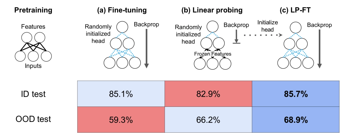
Average accuracies (10 distribution shifts)
So, as expected, FT achieves higher accuracy than probing on ID data. However, the opposite is true for OOD data: linear probing performs better for the OOD distribution, meaning it generalizes better.
There’s a clear explanation for this. During probing, we don’t change the pretrained weights - we gradually “slide” toward the optimum for the downstream task, but we never fully converge, since we’re only training the classification head.
In contrast, when we fine-tune the full model, the head’s random initialization causes gradients to shift the model weights too much in the early iterations. This leads to overfitting.
A simple solution to the drawbacks of both approaches is first to train the head, and then, with this pre-trained head, we will perform full fine-tuning (LP-FT). It turns out that LP-FT allows you to win on both ID and OOD data.
Adaptive PEFT
We have already realized that full fine-tuning is very expensive, as it requires storing gradients for all model weights in memory. This is where PEFT comes in - a method that fine-tunes only a minimal subset of parameters. It’s commonly used to train LLMs, which are too computationally expensive to train entirely.
A significant advantage of this approach is that, when fine-tuning on multiple different downstream tasks, you only need to store the small set of modified parameters for each task (this is exactly what OpenAI does for its SFT API)
Prompt tuning vs Prefix tuning
Prompt tuning is an approach where we aim to automatically select the most suitable prompt by optimizing only a set of learnable prompt embeddings, which are concatenated with the input sequence (the pretrained model remains frozen).
There are several ways to initialize prompt embeddings. The most common is random initialization trained from scratch. A more advanced method uses embeddings from the model's vocabulary. For classification tasks, we can initialize embeddings with target class tokens — similar to verbalizers — which can help constrain the model's output to valid classes.
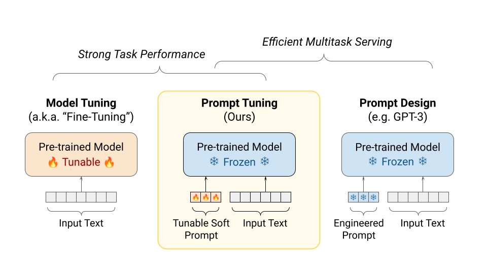
Comparison of fine-tuning, prompt tuning, and prompt design strategies for LLMs
The original paper presented comparisons of prompt tuning scaling. As expected, the prompt size directly impacts the quality, but the larger the model, the smaller the difference in quality. The disadvantage of prompt tuning is the instability of training: the quality changes non-monotonically with increasing prompt and model sizes. Also, the trained prompt limits the context window and slows down the model.
Prefix tuning is often confused with prompt tuning. A small set of task-specific vectors is also trained here, but instead of being added to the input sequence, they are injected into each transformer layer. The prefix consists of a few learnable key and value vectors per layer, which are shared across all attention heads within that layer. Disadvantages include low effectiveness on small models (as with prompt tuning) and the architectural modifications.
Adapters
This is a series of methods that add something to the model. The idea is as follows: after each attention and FFN layer, a small trainable adapter is added. It has a skip-connection and two fully-connected layers with a dimensionality reduction (to reduce the number of parameters). Only the adapters, layer normalization, and the final classification head are trained; all other parameters remain frozen.
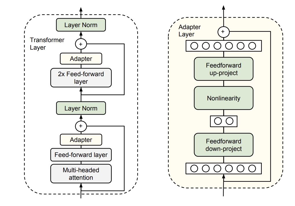
Adapter layer architecture
However, the basic version of the adapter adds quite a lot of parameters compared to prompt tuning. Moreover, adapters introduce additional layers that can’t be computed in parallel (because they are sequential blocks, which slow down the model’s inference).
LoRA
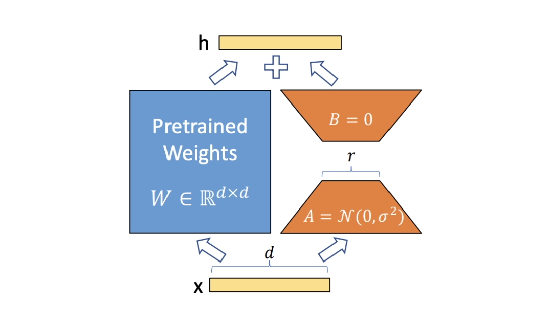
LoRA mechanism
An upgrade to adapters can be considered the LoRA method. We know that to adapt the model to a new downstream task, we need to shift the weights towards the antigradient:
W′ = W + ΔW
Let’s approximate W by the product of the low-rank trainable matrices BA (in the original paper, this method was applied only to the query Wq and value Wv weight matrices of the attention layers).
W′ = W + (α / r) · B A
Matrix A is initialized randomly (typically Gaussian), with small values (e.g., scaled by 0.01). Matrix B is initialized to zero, so the initial output is exactly the same as the frozen model (ensures stable training start).
Thus, very few parameters are added, and the update can be computed in parallel with the original model forward pass (unlike adapters). Currently, this is the most popular method of PEFT.
rs-LoRA
While LoRA works well for small ranks (e.g., 4, 8), it performs poorly when rank r is large. As was shown in research, higher-rank LoRA adapters don't improve performance. This happens because dividing by r makes gradients collapse when r increases. The model essentially “wastes” the extra capacity, since updates become too small to be effective.
rs-LoRA (rank-stabilized LoRA) is a corrected formulation that fixes the scaling factor to prevent gradient collapse. The paper proves that to remain learning stable, the scaling factor should be defined as:
γᵣ = α / √r
With rs-LoRA, larger ranks (e.g., 128, 512) give better perplexity and fine-tuning results.
FourierFT
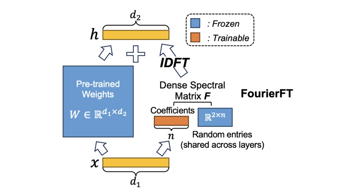
FourierFT mechanism
FourierFT is another lightweight fine-tuning method that encodes weight updates in the frequency domain. Instead of learning low-rank matrix adaptation (as in LoRA), it learns a small set of trainable spectral coefficients c, corresponding to a sparse subset of 2D Fourier frequencies (shared across layers). These coefficients are mapped into the full update matrix W using an inverse discrete Fourier transform (IDFT), followed by scaling and projection back to the real domain:
w′ = w + α R{ 𝓕⁻¹(E ⊙ c) }
where E represents the frozen spectral entries, c is the set of learnable spectral coefficients, ⊙ it’s the element-wise operation to create the spectral matrix, 𝓕⁻¹ is the IDFT, R is the real part of the transformed data, and alpha is a scaling factor.
Obviously, FourierFT has far fewer trainable parameters than LoRA because it learns just one real coefficient per selected frequency per layer, instead of full low-rank matrices. All layers share the same list of frequency indices (the shared index map), which further reduces memory. As a result, FourierFT can use up to 20× fewer parameters than LoRA. Also, the Fourier basis (made of sine and cosine waves) captures structure more effectively than random or generic orthogonal bases.
The main drawbacks include the need to manually select spectral indices and tune hyperparameters. The appendix of the original paper provides tables for various tasks where these parameters vary significantly. Additionally, 2D IDFTs are used during training, which involve complex values; while this is efficient on GPUs, it adds complexity to implementation and debugging.
VeRA
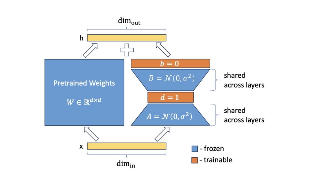
VeRA mechanism
VeRA or Vector-based Random Matrix Adaptation is a method that adds a parallel processing path in the attention block’s linear layers using fixed, randomly initialized rank matrices, similar to LoRA. These matrices are sampled once (e.g., Kaiming initialization) and shared across layers, remaining frozen during training. VeRA introduces two learnable scaling vectors that, when multiplied by the frozen matrices, facilitate downstream adaptation:
w' = w + Λb·B·Λd·A
Here, B and A are the frozen rank matrices, and b and d are the learnable scaling vectors (used as diagonal matrices) for matrices B and A, respectively.
As you understand, VeRA requires significantly fewer trainable parameters than LoRA. While the original paper reports that VeRA achieves comparable performance to LoRA, in practice, since VeRA only fine-tunes per-layer scaling vectors applied to frozen low-rank matrices, the rank of these frozen matrices often needs to be much higher than in LoRA to achieve similar results. This trade-off reflects the limited adaptability of fixed random projections compared to fully trainable low-rank adapters.
Selective PEFT
BitFit
BitFit stands for bias-terms fine-tuning, and the idea of the method comes directly from its name. In the model, we have many linear layers consisting of weight matrices and bias vectors. Since the biases contain few parameters, let’s train only them.

This picture highlights the bias terms (shown in red) that are trained in BitFit. All other parameters (e.g., weights, attention projections) remain frozen
This approach relies on the hypothesis that pre-trained models already encode powerful representations, and only small task-specific shifts (captured through bias changes) are needed for effective transfer.
It’s the lightest PEFT method (except prompt tuning). BitFit performs competitively on many NLP tasks, especially when the pre-trained model’s representations align well with the target domain. However, its limited parameter space restricts its expressiveness, which can lead to underperformance on complex tasks or when significant domain shifts are present.
LayerNorm Tuning
LayerNorm Tuning is another selective PEFT technique that freezes every weight in the backbone model except the two parameters (scale γ and shift β) of each LayerNorm layer inside the attention blocks. The model can learn to normalize activations across different tasks better, potentially stabilizing training and improving performance.
However, the method is limited: it can be applied only to the model that uses LayerNorm layers. Additionally, because only the scaling factors are tuned, LayerNorm-based adaptation may lack the expressive capacity needed for large-scale domain shifts. Its performance also tends to plateau when exposed to larger datasets.
Benchmarking PEFT Strategies
Most PEFT methods are implemented in the HuggingFace library of the same name. It is a very convenient tool for ML engineers, as it allows the use of a unified pipeline for different fine-tuning methods.
We decided to compare the previously reviewed efficient fine-tuning strategies on the most popular downstream task — text classification. As the dataset, we used MRPC from the GLUE benchmark (a dataset created by Microsoft Research for paraphrase identification). As the base model, we chose one of the smallest open-source MoE models — Qwen3-0.6B. Training experiments were conducted using Modal cloud GPU environments (A100 40GB).
We evaluated the results based on the number of trainable parameters, actual training time, GPU utilization, and classification metrics. You can run the same experiments by cloning our public repository on GitHub.
Pay attention that the performance of a given method depends on the specific downstream task and dataset. Training, optimizer, and scheduler hyperparameters also play a significant role. We used the hyperparameter setup recommended by the authors in the original paper for classification tasks.
| Method | Trainable params % | GPU utilization % | Time (s) | Val F1 | Val ROC AUC |
Linear Probing | 0.000003% | 70.57% | 134 | 0.8014 | 0.6832 |
BitFit | 0.000005% | 75.01% | 150 | 0.8178 | 0.7739 |
LayerNorm tuning | 0.01% | 91.06% | 161 | 0.8371 | 0.8157 |
Prompt tuning | 0.0001% | 92.88% | 196 | 0.801 | 0.558 |
Prefix tuning | 0.05% | 86.18% | 181 | 0.8107 | 0.572 |
LoRA | 0.38% | 66.44% | 264 | 0.8841 | 0.9203 |
rs-LoRA | 0.38% | 78.02% | 247 | 0.9155 | 0.9353 |
VeRA | 0.0004% | 68.29% | 263 | 0.8188 | 0.7833 |
FourierFT | 0.02% | 74.59% | 231 | 0.9058 | 0.9335 |
BitFit couldn't be properly trained, as the Qwen architecture doesn't include bias terms in the attention blocks. As a result, only the biases in the layer norm layers and the classification head’s bias were trainable. Additionally, the performance of the Adapters method is not shown in the table, as it is considered deprecated in the PEFT library (supported only for the first LLaMA and Mistral-7B models).
Conclusion
- So, FourierFT emerged as the most effective lightweight tuning method, achieving the highest validation performance while updating only 0.02% of the model parameters.
- rs-LoRA stands out as the strongest overall performer. It achieved the highest validation scores while keeping the same parameter footprint as standard LoRA (0.38%).
- Standard LoRA remains a strong third choice. Its performance rivalled FourierFT and required more trainable parameters and the longest training time. When GPU memory is enough and plug-and-play integration matters more than metrics, LoRA is still a robust default.
- If you are memory- or storage-bound, LayerNorm tuning or BitFit still unlock gains over linear probing.
- Prompt- and prefix-tuning underperformed. Despite high GPU utilization, their metrics plateaued near the linear-probe baseline. This confirms earlier findings that input-based tuning methods are less effective on smaller models and can slow down inference because they increase the input sequence length.
- VeRA occupies a middle position: it has a parameter count similar to BitFit, training time similar to LoRA, and quality between the two. Its frozen random projections appear less expressive than LoRA’s trainable low-rank subspaces, confirming the adaptability-rank trade-off discussed earlier.


Author